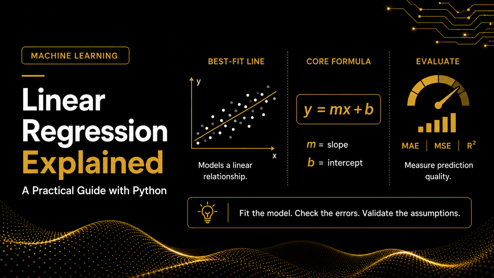
Linear regression connects input features to a continuous numeric outcome through a best-fit line or hyperplane.

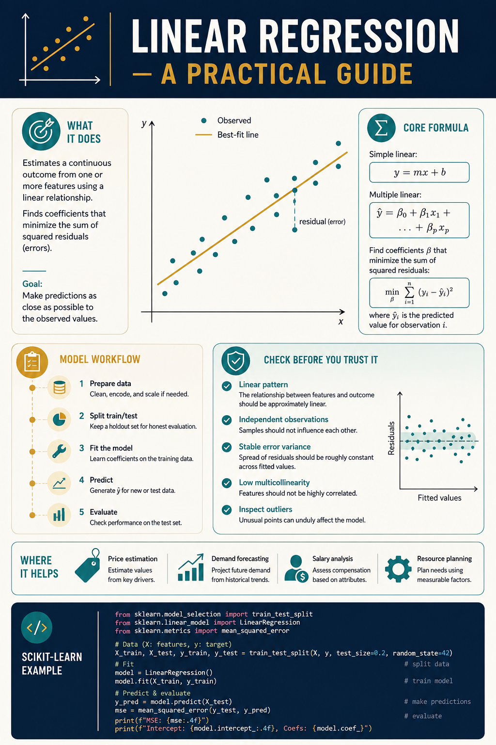
Linear regression is one of the most useful starting points in data science. It is easy to explain, quick to train, and valuable when a business wants to estimate a numeric outcome such as a house price, monthly sales, salary, demand, or fuel consumption.

What Is Linear Regression?

Linear regression is a supervised machine-learning algorithm used for regression problems. A regression problem has a continuous numeric target. For example, predicting a price of $425,000 is a regression task, while predicting whether a customer will churn is a classification task.

In simple linear regression, one feature is used to predict the target:

• y is the predicted target.
• x is the input feature.
• m is the slope—the expected change in y when x increases by one unit.
• b is the intercept—the predicted value of y when x is zero.

Multiple linear regression uses several input features:

Each coefficient measures the expected change in the target associated with its feature while the other included features remain constant.

How Does the Best-Fit Line Work?

The model chooses coefficients that make its predictions as close as possible to the observed values. The vertical difference between an observed value and its prediction is called a residual.

Ordinary least squares fits the model by minimizing the sum of squared residuals. Squaring prevents positive and negative errors from cancelling each other and gives larger errors more influence.

A Practical Modeling Workflow

1. Prepare data
   Clean values and select useful features.
2. Split data
   Keep test records separate.
3. Fit model
   Learn coefficients from training data.
4. Predict
   Estimate targets for unseen records.
5. Evaluate
   Measure error and validate assumptions.

Build Linear Regression in Python

The following example predicts sales from advertising spend. The data is intentionally small so beginners can understand each step.

import pandas as pd
from sklearn.model_selection import train_test_split
from sklearn.linear_model import LinearRegression
from sklearn.metrics import mean_absolute_error, mean_squared_error, r2_score

data = pd.DataFrame({
    "advertising_spend": [10, 15, 20, 25, 30, 35, 40, 45, 50, 55],
    "sales": [22, 28, 35, 39, 47, 52, 58, 65, 69, 76]
})

X = data[["advertising_spend"]]
y = data["sales"]

X_train, X_test, y_train, y_test = train_test_split(
    X, y, test_size=0.20, random_state=42
)

model = LinearRegression()
model.fit(X_train, y_train)

y_pred = model.predict(X_test)

print("Intercept:", round(model.intercept_, 2))
print("Slope:", round(model.coef_[0], 2))
print("MAE:", round(mean_absolute_error(y_test, y_pred), 2))
print("MSE:", round(mean_squared_error(y_test, y_pred), 2))
print("R-squared:", round(r2_score(y_test, y_pred), 2))

Example output

Intercept: 10.14
Slope: 1.20
MAE: 0.75
MSE: 0.88
R-squared: 1.00

Your output can vary when you change the data, test size, or random state. The important skill is understanding what each result means.

How to Interpret the Results

Metrics Used to Evaluate the Model

Assumptions to Check

• Linear relationship: the average relationship between the predictors and target should be approximately linear.
• Independent observations: one observation should not improperly influence another.
• Stable error variance: the spread of residuals should remain roughly constant across fitted values.
• Low multicollinearity: predictors should not be excessively correlated with one another.
• Residual normality: approximately normal residuals matter mainly for reliable confidence intervals and hypothesis tests.
• Influential points: outliers and high-leverage records should be investigated rather than automatically removed.

Advantages and Limitations

Real-World Business Applications

• Real estate: estimate property prices using size, location, condition, and age.
• Human resources: analyze how experience, role, education, and skills relate to compensation.
• Retail: forecast sales or demand using price, promotions, seasonality, and historical performance.
• Operations: estimate resource usage, delivery time, fuel consumption, or production cost.
• Agriculture: study how rainfall, temperature, soil conditions, and inputs relate to crop yield.

Common Beginner Mistakes

1. Using linear regression when the target is a category rather than a number.
2. Evaluating the model on the same data used for training.
3. Assuming correlation or a coefficient proves causation.
4. Ignoring missing values, outliers, leakage, and unrealistic records.
5. Reporting a high R² without checking prediction errors and residual patterns.
6. Making predictions far outside the range represented in the training data.