
Statistics is the backbone of data analysis, providing the tools necessary to uncover patterns and make predictions based on data. One of the most powerful concepts in statistics is the understanding of discrete distributions. These distributions help us model and analyze situations where the data takes on distinct, countable values. In this article, we will explore the world of discrete distributions, focusing on two key players: the Binomial distribution and the Poisson distribution. By the end of this exploration, you’ll have a solid understanding of how these distributions work, when to use them, and how they can make sense of real-world data.
What is a Discrete Distribution?
At its core, a discrete distribution refers to the probability distribution of a discrete random variable—a variable that can take on only specific, countable values. Unlike continuous variables (which can take on any value within a given range), discrete variables are confined to a finite set of possible outcomes. For example, the number of heads in a series of coin flips or the number of defective items in a batch of products are discrete variables.
A discrete distribution tells us how the probability of different outcomes is spread across the possible values of a random variable. This distribution can be described by a probability mass function (PMF), which assigns probabilities to each possible value of the variable.
The Binomial Distribution: Modeling Success and Failure
The Binomial distribution is one of the most commonly used discrete distributions in statistics. It is used to model the number of successes in a fixed number of trials, where each trial has only two possible outcomes—commonly referred to as “success” and “failure.” Think of a coin toss: each toss results in either heads (success) or tails (failure).
Key Parameters of the Binomial Distribution:
- n: The number of trials or experiments.
- p: The probability of success on each trial.
- k: The number of successes we are interested in.
- q = 1 – p: The probability of failure on each trial.
The Binomial distribution is represented as Binomial(n, p), where:
- n is the number of trials,
- p is the probability of success on each trial.
The formula for the Binomial probability mass function (PMF) is:
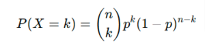
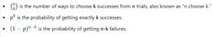
Where:
Example: Tossing a Coin
Let’s say you flip a coin 5 times and want to find the probability of getting exactly 3 heads. In this case:
- n = 5 (5 coin flips),
- p = 0.5 (the probability of heads),
- k = 3 (we want exactly 3 heads).
Using the Binomial formula:
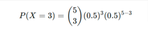
After calculation, we would find the probability of getting exactly 3 heads out of 5 flips.
When to Use the Binomial Distribution:
The Binomial distribution is used when:
- You have a fixed number of trials (n).
- Each trial has two possible outcomes (success or failure).
- The probability of success is the same for each trial (p).
- The trials are independent of each other.
Some real-world examples include:
- Quality control: Counting the number of defective items in a batch of products.
- Survey research: Determining the number of respondents who agree with a particular statement out of a fixed sample.
- Medical trials: Tracking the number of patients who respond to a treatment out of a fixed group.
The Poisson Distribution: Modeling Rare Events
The Poisson distribution is another essential discrete distribution in statistics. It is used to model the number of events that occur in a fixed interval of time or space, where the events happen independently of each other. Unlike the Binomial distribution, the Poisson distribution does not require a fixed number of trials, but rather models the count of events over a continuous interval.
Key Parameters of the Poisson Distribution:
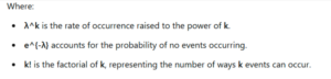
- λ (lambda): The average rate of occurrence of events within a given interval (mean).
- k: The number of events that actually occur in the interval.
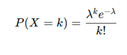
The Poisson distribution is represented as Poisson(λ), and the PMF is given by:
Example: Call Center Analysis
Imagine a call center that receives an average of 10 calls per hour. The Poisson distribution can be used to determine the probability of receiving exactly 7 calls in an hour. Here:
- λ = 10 (average number of calls),
- k = 7 (desired number of calls).
Using the Poisson formula:
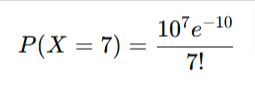
After solving this, you’ll get the probability of receiving exactly 7 calls.
When to Use the Poisson Distribution:
The Poisson distribution is appropriate when:
- Events occur independently of each other.
- The events happen at a constant average rate over time or space.
- The number of events in a given interval is countable but can vary.
Some real-world examples include:
- Traffic flow: Modeling the number of cars passing through a toll booth in an hour.
- Internet traffic: Estimating the number of website visitors in a given period.
- Accident analysis: Counting the number of accidents occurring at a particular intersection over a set period.
Comparing Binomial and Poisson Distributions
Although both distributions model the count of events, they are used in different scenarios:
- The Binomial distribution is used when there is a fixed number of trials (n), and each trial has a constant probability of success (p).
- The Poisson distribution is used when we are interested in the count of events happening in a continuous interval, with a known average rate of occurrence (λ).
However, there is a connection between them: when n is large, and p is small (such that np = λ), the Binomial distribution can approximate the Poisson distribution. This is particularly useful when modeling rare events.
Conclusion: The Power of Discrete Distributions
Discrete distributions are a cornerstone of statistical analysis. Whether you are examining the number of successes in a fixed number of trials (Binomial distribution) or the occurrence of rare events over time (Poisson distribution), these tools help you unlock the patterns behind your data.
By understanding when and how to apply these distributions, statisticians can make sense of count-based data, predict outcomes, and make informed decisions across various fields, from business and healthcare to engineering and marketing. The next time you encounter a scenario where events are countable or binary, you’ll know exactly which distribution to turn to.
Embrace the power of discrete distributions, and let them guide you in unlocking the secrets hidden in your data!